Quick Start

Installation

Package installation: pip install azapyGUI

Start

To start the application, you need to write the following 2-line python script. For this example, let’s call it my_azapy.py.

import azapyGUI
azapyGUI.start()

Then run the script in a powershell as

python my_azapy.py

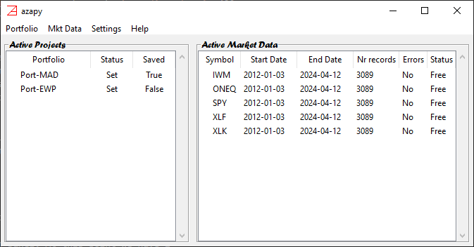
This will bring up the main application panel.

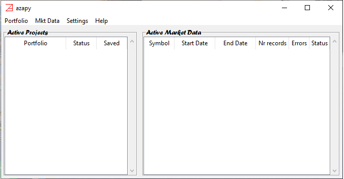
There are no active projects nor active market data for now. We will come back to these in a minute. For now, first things first.

Basic Setups

On the menu, click on Settings and then on Application Settings. The User Default Settings window will popup.

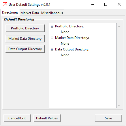
In the first tab, called Directories, you must make three choices.

1. Portfolio Directory - this is the default user directory where you can save/load portfolio/project files. When save/load a project, you will be prompted to this directory (you can always change it).

2. Market Data Directory - local (buffer) market data directory. Once the historical data is retrieved form the provider, a copy is stored in this directory. Successive calls for the same market data will try first to access data from this directory and then, and only if there is a need to update the data, from the provider. This will speed up considerable the computations (in general accessing repeatedly the same provider data over the internet may add up to a considerable amount of time). The market data stored in this directory is not intended to be consumed by other applications nor as permanent storage. There are other mechanisms provided by azapyGUI for visualizing and analyzing the market data as well for saving it in a variety of file formats.

3. Data Output Directory - this is the default user directory where graphical and analytical reports can be saved for further inspection.

Then press Save and close the window.

These are persistent setups, preserved between azapyGUI sessions.

By default, azapyGUI is set for NYSE products. If you are interested in working with equity products from non-US exchanges please see here additional information.

We will come back later to the topic of application settings with more details about the available options. For now, this is all what we need to start the very first azapyGUI session.

Build First Portfolio

Now we are back at the main panel, and we will start to build the first portfolio project. On the menu, click the tab Portfolio and then click on item New.

A Portfolio Edit window will popup.

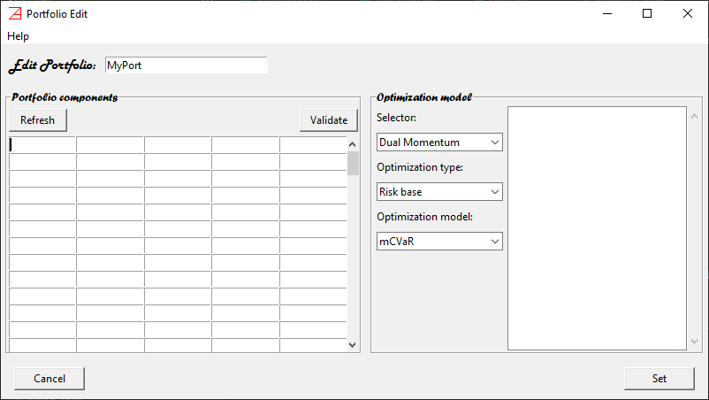
Here we will enter the portfolio information: name, components, and optimization model.

1. Name - on the entry space, right of label Edit Portfolio, replace the suggestion MyPort with the name you want for this portfolio (try to choose something short and meaningful for you). For our example let us type Port-MAD. I know, it is not very inspiring or meaningful, but it will help us to navigate this example.

2. Portfolio Components - on the left panel enter the symbols of the portfolio components. For our example let’s type SPY, ONEQ, IWM, XLK, and XLF. You must enter one symbol name per cell. It doesn’t matter in what order, lower or upper case, or in what specific cell. Then press the Refresh button. The symbols will be enumerated in alphabetical order, upper case, from left to right and up to down. Also, entries with special characters that cannot be present in a valid symbol name will be eliminated silently. This is a good time to check the spelling too. In our case, the 5 symbols belong to 5 very popular ETF’s. However, to make sure that they are valid market symbols for our market data provider, let’s press on the Validate button. A Symbols Validation window will popup.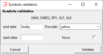

   

   We will discuss later the optional entries in this window. For now, just notice that the market data provider is yahoo. It is our default choice (it is free “as is”). Later, we will discuss how other (pay for) market data providers can be set up. Let’s press on the Validate button. You will notice two things.

   • It takes a while to release the window. This is the time spent by azapyGUI to contact the market data prover (in our case yahoo) and to make a minimal request for 1 (most recent) historical record for each of the symbols. In this way it establishes that these symbols are valid market shares symbols, and they can be used in defining our portfolio.

   • The right side of application main panel, Active Market Data was populated with our symbols (although the length of the historical data is only 1 day - hardly enough for any computations).

3. Optimization Model - although there are many and some of them very complex choice, for this example we will make a simple choices. On the third drop-down list under the label Optimization Model: click on mMAD (mixture Mean Absolute Deviation). An mMAD edit model parameter window will popup.

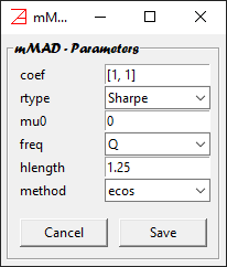
We will comment later on the meaning of these parameters. For now, we will accept the default values. They stand for maximization of Sharpe ratio with 0 risk free rate and (1,1)-mMAD risk measure, targeting quarterly rates of return for a look-back period of 1.25 years, using the ecos numerical library for LP (linear programming) problems. Let’s press on the Save button. The model parameter window will close and our model will appear in the right panel of Portfolio Edit window. By pressing on + it can be extended to view the value of all parameters.

At this point we are almost done. What is left is to press on the Set button. The Portfolio Edit window will close and our model will be visible in the left panel of main application window. It will have.

• Status::Set - it means that the portfolio is ready for computations.

• Save::False - it means that the portfolio is not yet saved. To save the portfolio, left click the mouse on the portfolio name. From the dropdown menu chose Save item and proceed to save the portfolio structure to a file in the default directory.

Backtesting

Now we are ready to put our portfolio to the test, i.e., backtest.

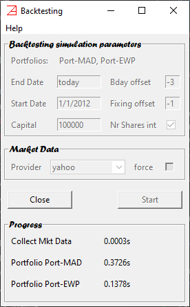
Left click the mouse on the portfolio name, and from the dropdown menu choose the Backtest item. The Backtesting window will popup.

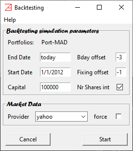
We will accept the default values. Later we will discuss in detail all available options. However, it is worth mentioning a few features now. The name of our portfolio is at the top of the screen. In general, azapyGUI allows for multiple portfolios backtesting. In this case the list of portfolio names will be visible at the top of the window. End date is set to today (i.e., most recent market closing date) and the start date is set to 1/1/2012 (i.e., the first market closing date after, and including, 1/1/2012). The rebalancing date is set to 3 business days before (this is the meaning of -3 value for Bday offset field) the end of the calendaristic quarter (the quarterly reset was defined by the model parameter, i.e., Q choice for freq value). The fixing date (i.e., the closing day relative to which the portfolio weights are computed) is defined as the closing day before the rebalancing day (i.e., the -1 value for Fixing offset field). A check of Nr Shares int box, stands for using whole numbers (opposed to fractional) of shares (therefore the portfolio will be subject to rebalancing round off errors - in practice they are very small).

Let’s press the start button. The backtesting process starts collecting the market data. It will take a bit of time to retrieve the data directly from the provider and a lot faster if it is already cached. Then the actual numerical computations will proceed (by default azapyGUI will use all CPU cores available). The effective user time for these process (market data collection and actual numerical evaluations) will be posted at bottom of the window. When all the computations are finished the Statistics window will popup.

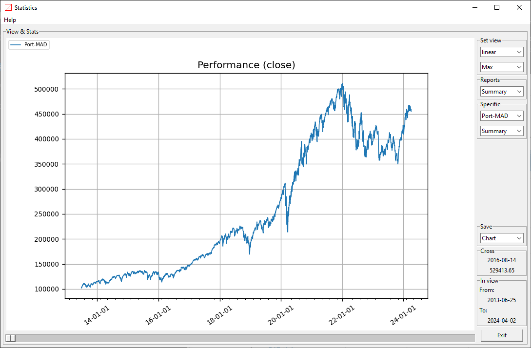
The plot is our portfolio performance over time, assuming full reinvestment. On the right side panel there are many graphical and analytical options (numerical reports). They will be discussed later. For now, let us look at the Specific section (i.e., portfolio specific analytic reports) and from the second dropdown entry click on Annual (i.e., the annual returns report). The Annual Report window will popup.

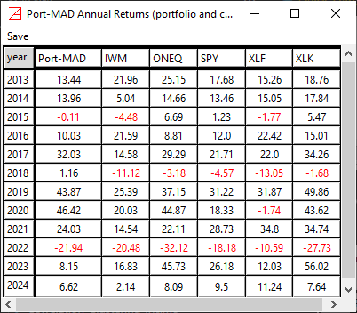
The portfolio and its components’ annual returns (percent) are presented. The negative returns are printed in red. Note that, pressing the year heading cell, the results will be printed in descendent order of years. To save this report, press on the menu save and choose the format. You will be prompted to save the report in the default location (defined in Setting Data Output Directory).

We will stop this presentation here, hoping that you have got a general idea about azapyGUI backtesting capabilities. Later, we will explore the full set of analytic reports.

Rebalancing

Another important azapyGUI functionality is the computation of weights and the size of buy/sale orders to rebalance an existing portfolio.

Let’s imagine that we are after today closing and tomorrow we would like to initiate a position in Port-MAD. We will need to compute the weights and the number of shares that we need to buy. To initiate these computations, let’s go back to the main panel, right click the mouse on the portfolio name, and select Rebalance item. The Rebalance window will popup.

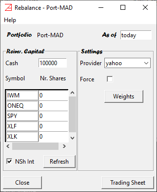
In the left panel are the components of our capital. Since this is a new position on this portfolio, we will start with a cash amount of money and zero shares. By default, in the Cash entry, it is printed 100000 (dollars). You can change this value to an actual amount of dollars you want to allocate to this investment. Then, if you press the Weights button, azapyGUI will return a report showing the value of the weights for each portfolio component. This is useful information to understand capital allocation. Further, if we press on the Treading Sheet button, the transactions report will popup. Here are listed the initial, final, and delta (final-initial) positions for all assets with non-zero allocations. This report can be saved and used next day (rebalancing day) to assist the execute of the actual transactions.

The similar computation for an existing portfolio requires to enter the initial (existing) number of shares for each portfolio component and a non-zero value for Cash only if we want to increase the capital (a positive amount) or reduce the capital (a negative value) for this strategy. Then, the Treading Sheet will show the right number of shares (delta positions) that will rebalance the portfolio.

Backtesting Multiple Portfolios

Another aspect of azapyGUI backtesting facility is the ability to handle multiple portfolios. It provides an easy way to compare several portfolio strategies. Although there are no limitations (besides hardware limitation in terms of memory and computational speed) in how many portfolios can be backtested at once, we fund that more than 20 in a single batch become hard to follow. Running multiple batches and sequentially eliminating the wicker candidates, is a more reliable selection strategy.

To illustrate this facility, in this example we will use only 2 portfolios. Let’s start by cloning our previous Port-MAD portfolio. On the main application window left click the mouse on the portfolio name and select the Clone items. A portfolio clone window will popup.

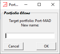
It is asking us to choose a name for the new portfolio. Let’s go ahead and type Port-EWP (soon will become clear why we chose this name). Then press OK. A new entry will appear in the Active Projects section of the main application panel. At this point we have 2 identical portfolios with different names. Let us edit Port-EWP. Left click the mouse on the portfolio name and select the Edit item. The portfolio edit window will popup. It will look as

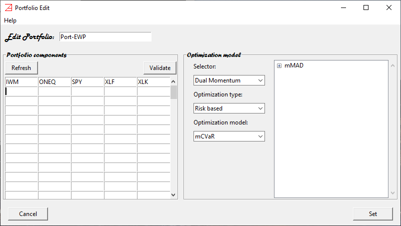
It is the same as for Port-MAD except the name is now Port-EWP. We would like to keep the same portfolio components and change the optimizer model. To do that let’s first remove the present optimization model mMAD. We can have only one optimizer associate with a given portfolio. To do that, on the right panel, Optimization model, left click the mouse on the model’s name and choose Delete item. The model’s name will disappear. Now it is time to choose another optimizer. Left click the mouse on the second combobox under the label Optimization type and choose Naive item. This will select the family of optimization models. Then, in the combobox below left click the mouse and choose the Equal Weighted item. The Equal Weighted model parameters window will popup

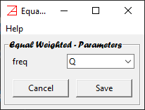
This is the simplest portfolio model, the Equal Weighted Portfolio (hence the name of our portfolio, Port-EWP). As the name suggests, the portfolio weights are periodically rebalanced to be the same for all components. The only parameter we need to choose is the rebalancing frequency. Let’s keep the default value Q, it stands for quarterly rebalance, and press the OK button. Now the Equal Weighted model is associated with our portfolio Port-EWP. As a side note, we should mention that the EWP, although very simple, is a popular benchmark portfolio often used to evaluate the goodness of a more sophisticated optimization scheme. Let’s go ahead and press the Set button. Even if we didn’t ask explicitly to validate the components symbols, azapyGUI will validate them with the market data provider. If the market data is not already cached, then this procedure may take a bit of time. Finally, we have 2 distinct portfolios waiting for us. If everything went well, the main application window should look like this.

Now press Shift + left click the mouse select both portfolio and from the popup menu click on Backtest item. Note that pressing Ctrl + left click the mouse will produce the same result in our case. In general pressing Shift will force a selection of consecutive items while Ctrl will limit the selection only to the item pointed by the mouse. Again the Backtesting window will popup with both portfolio names listed at the top. We choose the default settings and press directly the Start button. The backtesting procedure will start by collecting the market data (for all portfolios) and then computing each portfolio independently. At the end of computations the Backtesting window will look like

You can notice the time spent (by my computer - an average configuration) collecting the market data and computing each portfolio. Also, a new Statistics window will popup.

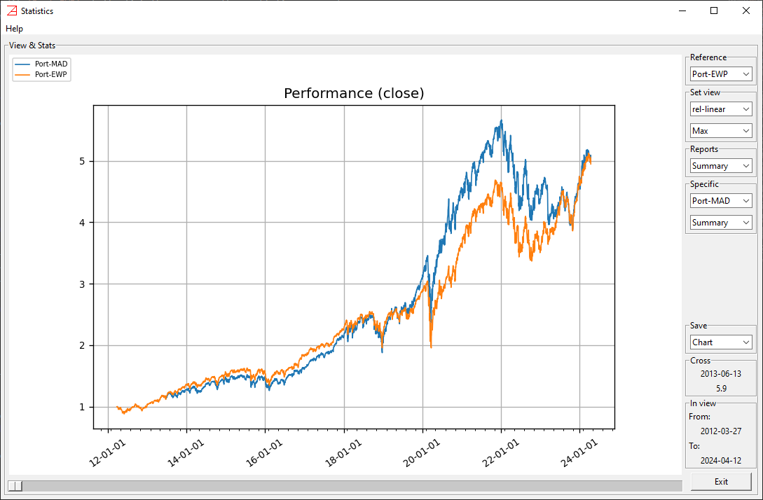
It is like the one before (for a single portfolio) but with a few more features. On the right side there is a new box called Reference. Since the time series for Port-MAD and Port-EWP have different lengths, the Reference combobox indicates the time series used as reference for the graphical presentation. The default choice is the longest time series. In our case Port-EWP. However, if you want to change the reference time series, just click on the desired one.

Note that, EWP model doesn’t need special calibration; all weights are equal to 1/n where n is the number of portfolio components. Therefore, the backtesting period starts immediately (at the first rebalancing date). For Port-MAD the backtesting period can start only after 1.25 years reserved for first calibration of portfolio weights (this value was set as a model parameter). Hence the uneven length of two series in our example.

All other features are the same. The Report box refers to comparative reports between the two portfolios, while the Specific box to portfolio specific reports. Every report, as well as the graph, can be saved as usual.

Example of a complex portfolio

To further illustrate the power of azapyGUI, let’s discuss an example of more complex portfolios, involving multiples selectors as well as an optimization model. The selectors will be presented in detail later. For now, we should keep in mind that they are analytical algorithms to restrict a given universe of a possible portfolio components to a smaller, eventually significant, number of candidates. While a selector may also put restrictions on the overall capital size, it will not define the portfolio weights. That job is reserved for the optimization model. In general, a portfolio model may be a collection of selectors followed by an optimizer. The order of selectors matters.

Without further due, let’s start to define our portfolio. From the menu choose the New item, to open the Edit window. Let’s name this portfolio Port-FT_MAD, and for components, let’s enter: BRK-B, DIA, HDV, ILV, ITA, IWF, IWM, IWV, ONEQ, QQQ, SPY, VGT, VHT, VIG, VTV, VUG, XAR, XBI, XHE, XHS, XLB, XLE, XLF, XLI, XLK, XLU, XLV, XLY, XRT, and XSW. In total there are 30 symbols. All are popular ETF’s, except BRK-B which is not an ETF. However, BRK-B behaves as a closed-end found, so it is OK to be in this list (I hope, I didn’t offend anybody’s feelings about BRK-B). On the Optimization model section let’s choose, from the top combobox, 2 selectors: Correlation Clustering and Dual Momentum. In both cases we accept the default parameter values. Latter we will discuss more the analytics behind these selectors and how they behave. For now, let’s keep in mind:

• Correlation Clustering will partition the universe of portfolio components in clusters with similar correlation (in our case higher than 0.98 - the default value). Then, from each cluster, it will choose, as a representative, the element with the higher weighted average of annualized, 1, 3, 6, and 12 months most recent rate of returns (also called f13612 filter).

• Dual Momentum will choose a maximum n components with positive f13612 filter value. The capital allocated to the risky assets (non-cash) is in full only if the total number of components with positive f13612 filter value is equal or greater than the threshold value m. Otherwise, the risky capital allocation will decrease proportionally, with the remainder reserved in cash (until the next portfolio rebalancing date). In our case n=3 and m=6 (the default values).

For optimizer model let’s choose as before the mMAD model with default parameters. The Edit window should look like this:

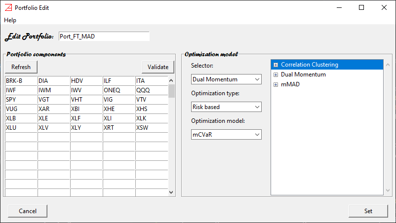
Note the order of the models. The optimizer is always the last (it is a hardcoded feature). The first selector is the Correlation Clustering. Strictly from a math point of view, it can also be in the second position. However, logically we want first to eliminate assets with similar correlations and then to choose by the best momentum value. So, we strongly prefer Correlation Clustering to be the first and Dual Momentum to be the second. If they are not in this order them left click the mouse in the selector name and choose to move it up or down as is the case.

Ok, let’s press on the Set button. If the components were not validated before then the validation is mandated in the background (so it may take a bit of time to set the portfolio).

By now, we have put a lot of work into defining this portfolio. So, let’s go ahead and save it before doing anything else.

Just to add a bit of spice to our example, let’s clone this portfolio to Port-FT_EWP, and as before, let’s change the optimizer of the newly cloned portfolio to Equal Weighted. Now we have 2 complex portfolios differentiated by the optimizer.

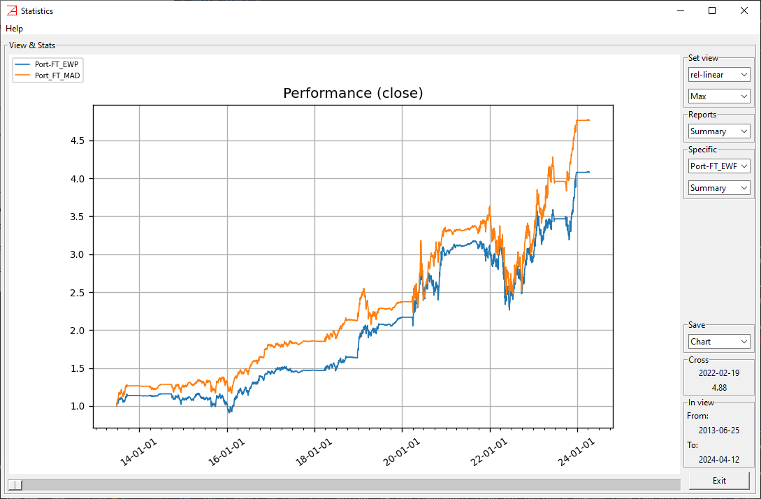
Select both portfolios and run the backtest. This is what I get running this example after the close on April 12th, 2024:

You can repeat these examples (finally using your choices for portfolio names) using different parameter values (e.g. f13612 filter weights, n=6 and m=12 for Dual Momentum thresholds, other optimizer models, etc.).